---
title: "arXiv has reached lift-off. Is it acceleration or slop?"
subtitle: "Where the surge in preprints is coming from, and what the metadata can and cannot tell us"
author: "Trey Saddler"
date: 2026-10-01
date-modified: 2026-10-02
categories: [arXiv, AI, Data Analysis]
jupyter: python3
format:
html:
toc: true
toc-depth: 2
code-fold: true
code-summary: "Show the code"
code-tools: true
fig-format: svg
fig-align: center
df-print: kable
include-in-header: arxiv-liftoff/assets/view-toggle.html
execute:
warning: false
---
A post on LinkedIn recently put the question plainly: monthly submissions to arXiv have "reached lift-off", and either AI has meaningfully accelerated research, or preprints are filling up with low-effort slop. How would we measure which is true? In the comments, Srijit Seal suggested a place to start: work out where the growth is coming from and how fast it is expanding, and check whether credible venues show the same explosion. If they do not, look for mills that "just submit papers every hour".
This article does that analysis with public data. Use the switch under the title to move between the takeaways and the full walkthrough, which shows how each dataset was fetched, every processing step, and the code behind every number.
::: {.callout-tip appearance="simple"}
**Updated 2 October 2026** with three questions from readers on LinkedIn. Was growth uniform across countries and university rankings? Do single-author papers mostly cite themselves? Is the new work being used, inside its own field and outside it? New sections: [Which countries and institutions](#which-countries-and-institutions), [Do solo authors cite themselves?](#do-solo-authors-cite-themselves) and [Is the new work being used?](#is-the-new-work-being-used).
:::
::: {.thorough}
The analysis is a single Quarto document running on the Jupyter kernel. This first cell sets up paths and one shared chart style.
:::
```{python}
#| label: setup
from pathlib import Path
import gzip, json, re, time, zipfile

import matplotlib.pyplot as plt
import matplotlib.ticker as mtick
import numpy as np
import orjson
import pandas as pd
import pyarrow.parquet as pq
import requests

DATA = Path("arxiv-liftoff/data")  # relative to posts/; not committed to the site repo
RAW, PROC = DATA / "raw", DATA / "processed"
PARTS = PROC / "parts"
for d in (RAW, PROC, PARTS):
    d.mkdir(parents=True, exist_ok=True)

UA = {"User-Agent": "arxiv-liftoff-analysis (mailto:treyosaddler@gmail.com)"}

# One visual system for every chart: thin marks, recessive axes, a fixed colour order.
BLUE, ORANGE, AQUA, YELLOW = "#2a78d6", "#eb6834", "#1baf7a", "#eda100"
INK, INK2, MUTED, GRID = "#0b0b0b", "#52514e", "#898781", "#e1e0d9"
plt.rcParams.update({
    "figure.figsize": (7.6, 3.9), "figure.facecolor": "#fcfcfb", "axes.facecolor": "#fcfcfb",
    "axes.spines.top": False, "axes.spines.right": False, "axes.spines.left": False,
    "axes.edgecolor": "#c3c2b7", "axes.grid": True, "axes.grid.axis": "y", "grid.color": GRID,
    "grid.linewidth": 0.8, "axes.axisbelow": True, "xtick.color": MUTED, "ytick.color": MUTED,
    "xtick.labelcolor": INK2, "ytick.labelcolor": INK2, "ytick.left": False, "font.size": 10,
    "axes.titlesize": 11, "axes.titleweight": "bold", "axes.titlelocation": "left",
    "axes.labelcolor": INK2, "text.color": INK, "lines.linewidth": 2, "legend.frameon": False,
    "svg.fonttype": "none",
})
thousands = mtick.FuncFormatter(lambda v, _: f"{v:,.0f}")
pct0 = mtick.PercentFormatter(1, decimals=0)
```
## The data {.thorough}
Seven public sources, each cached under `data/raw/` the first time it is fetched so that re-rendering does not hit anyone's servers again.
| Source | What it gives us | How it is fetched |
|---|---|---|
| [arXiv monthly submission statistics](https://arxiv.org/stats/monthly_submissions) | Official count of new submissions per month since 1991 | One CSV download |
| [arXiv metadata snapshot on Kaggle](https://www.kaggle.com/datasets/Cornell-University/arxiv) | One JSON record per paper: submitter, authors, categories, versions, comments, abstract | One 1.8 GB zip (5.6 GB of JSON lines) |
| [bioRxiv](https://api.biorxiv.org/) and medRxiv summary APIs | New preprints per month on the two largest life-science servers | One JSON call each |
| [Crossref REST API](https://api.crossref.org/) | Number of journal articles registered, by publication month | One count query per month |
| [OpenAlex](https://openalex.org/) | Author affiliations and countries for a random sample of arXiv papers | 50 paged requests per year sampled |
| [CWTS Leiden Ranking Open Edition 2025](https://open.leidenranking.com/) | Research indicators for 2,831 universities, keyed to OpenAlex institution ids | Three small tables read out of the [Zenodo archive](https://zenodo.org/records/17471989) |
| [Semantic Scholar](https://www.semanticscholar.org/product/api) | Reference lists and citing papers, with author ids and fields of study | Batch requests of 100 papers |
### Step 1: the small sources
```{python}
#| label: fetch-small
def fetch(url, name):
    """Download `url` to data/raw/`name` once; later runs reuse the cached copy."""
    path = RAW / name
    if not path.exists():
        r = requests.get(url, headers=UA, timeout=120)
        r.raise_for_status()
        path.write_bytes(r.content)
    return path

official = pd.read_csv(fetch("https://arxiv.org/stats/get_monthly_submissions", "arxiv_monthly_submissions.csv"))
official["month"] = pd.PeriodIndex(official["month"], freq="M")
official = official.set_index("month")["submissions"]

def rxiv_monthly(server):
    j = json.loads(fetch(f"https://api.{server}.org/sum/m", f"{server}_monthly.json").read_text())
    key = next(k for k in j if "statistics" in k)
    d = pd.DataFrame(j[key])
    return pd.Series(d["new_papers"].astype(int).values, index=pd.PeriodIndex(d["month"], freq="M"), name=server)

biorxiv, medrxiv = rxiv_monthly("biorxiv"), rxiv_monthly("medrxiv")
official.tail(4).to_frame()
```
The official arXiv series ends with a partial month (the file was pulled on 1 October 2026), so everything below stops at the last complete month.
### Step 2: journal output from Crossref
Crossref is the DOI registry most journals use. Asking for zero rows with a filter returns just the count of matching records, so one polite request per month gives a monthly series of journal articles by publication date. The loop is resumable: each answer is written to the CSV straight away.
```{python}
#| label: fetch-crossref
def crossref_monthly(kind="journal-article", start="2015-01", end="2026-09"):
    path = RAW / f"crossref_{kind}_monthly.csv"
    have = pd.read_csv(path) if path.exists() else pd.DataFrame(columns=["month", "count"])
    rows, seen = have.to_dict("records"), set(have["month"])
    for m in pd.period_range(start, end, freq="M"):
        if str(m) in seen:
            continue
        flt = f"type:{kind},from-pub-date:{m.start_time:%Y-%m-%d},until-pub-date:{m.end_time:%Y-%m-%d}"
        r = requests.get("https://api.crossref.org/works", params={"rows": 0, "filter": flt}, headers=UA, timeout=120)
        r.raise_for_status()
        rows.append({"month": str(m), "count": r.json()["message"]["total-results"]})
        pd.DataFrame(rows).to_csv(path, index=False)
        time.sleep(0.2)
    out = pd.DataFrame(rows)
    return pd.Series(out["count"].values, index=pd.PeriodIndex(out["month"], freq="M"), name="journals").sort_index()

journals = crossref_monthly()
journals.groupby(journals.index.month).mean().round(-3).astype(int).rename("mean articles by calendar month").to_frame().T
```
One artefact matters later: records with only a publication year are counted on 1 January, so January is roughly double any other month. Comparisons involving Crossref therefore use February to August only.
### Step 3: the per-paper metadata
The official statistics say how many papers arrived. To say *where from* and *who from*, we need one row per paper. arXiv's own OAI-PMH interface serves that, but at roughly 1,300 records per two-minute request a full harvest of three million records would take days. Cornell publishes the same metadata as a regularly refreshed snapshot on Kaggle, which downloads in a few minutes.
```{python}
#| label: fetch-kaggle
KAGGLE_ZIP = RAW / "arxiv-metadata-kaggle.zip"
if not KAGGLE_ZIP.exists():
    url = "https://www.kaggle.com/api/v1/datasets/download/Cornell-University/arxiv"
    with requests.get(url, stream=True, timeout=600) as r:
        r.raise_for_status()
        with open(KAGGLE_ZIP, "wb") as fh:
            for chunk in r.iter_content(1 << 22):
                fh.write(chunk)

with zipfile.ZipFile(KAGGLE_ZIP) as z:
    info = z.infolist()[0]
print(f"{info.filename}: {info.file_size/1e9:.1f} GB, snapshot written {info.date_time[0]}-{info.date_time[1]:02d}-{info.date_time[2]:02d}")
```
### Step 4: from 5.6 GB of JSON to a slim table
Each line of the snapshot is one paper. We keep only what the analysis needs and never unzip the file to disk: the records are streamed out of the archive, reduced to fifteen fields, and written as parquet parts of 400,000 papers each. Parts that already exist are skipped, so an interrupted run picks up where it stopped.
What each derived field means:
- `created` is the timestamp of version 1, the original submission. This matches how arXiv counts monthly submissions.
- `primary` is the first listed category; `n_cats` counts cross-lists.
- `submitter` is the display name of the account that uploaded the paper. It is a name, not an ID (see the limitations).
- `n_authors` comes from arXiv's own parsed author list.
- `accepted` flags comments that mention acceptance, publication or proceedings.
- `llm_marker` flags abstracts using any of a handful of words that LLMs of 2023 and 2024 were known to overuse.
```{python}
#| label: parse-fn
PAPERS = PROC / "papers.parquet"
COLS = ["id", "created", "n_versions", "primary", "n_cats", "submitter", "first_author", "n_authors",
        "has_jref", "has_doi", "accepted", "n_pages", "abs_words", "llm_marker"]

MARKERS = re.compile(r"\b(delv(e|es|ed|ing)|underscor(e|es|ed|ing)|showcas(e|es|ed|ing)|pivotal|intricate|meticulous(ly)?)\b", re.I)
PAGES = re.compile(r"(\d{1,4})\s*pages?\b", re.I)
ACCEPTED = re.compile(r"accepted|to appear|published|proceedings|camera[- ]ready", re.I)

def parse_record(d):
    cats = d["categories"].split()
    authors = d["authors_parsed"]
    comments = d["comments"] or ""
    pages = PAGES.search(comments)
    return (
        d["id"], d["versions"][0]["created"], len(d["versions"]), cats[0], len(cats),
        d["submitter"] or "", (authors[0][0] + ", " + authors[0][1]).strip(", ") if authors else "",
        len(authors), bool(d["journal-ref"]), bool(d["doi"]), bool(ACCEPTED.search(comments)),
        int(pages.group(1)) if pages else -1, len(d["abstract"].split()), bool(MARKERS.search(d["abstract"])),
    )

def part_done(k):
    """A part counts as done if it exists and was written with the current set of columns."""
    p = PARTS / f"part-{k:03d}.parquet"
    return p.exists() and pq.read_schema(p).names == COLS

def parse_snapshot(zip_path=KAGGLE_ZIP, chunk=400_000, budget_s=None):
    """Stream the snapshot and write one parquet part per `chunk` records. Returns True when complete.
    `budget_s` stops cleanly after that many seconds, for environments with short time limits."""
    t0, rows, part = time.time(), [], 0
    flush = lambda: pd.DataFrame(rows, columns=COLS).to_parquet(PARTS / f"part-{part:03d}.parquet", index=False)
    with zipfile.ZipFile(zip_path) as z, z.open(z.infolist()[0]) as f:
        have = part_done(part)
        for i, line in enumerate(f):
            if i and i % chunk == 0:
                if not have:
                    flush()
                rows, part = [], part + 1
                have = part_done(part)
                if budget_s and not have and time.time() - t0 > budget_s:
                    return False
            if not have:
                rows.append(parse_record(orjson.loads(line)))
        if not have:
            flush()
    return True
```
The last piece of cleaning is the subject grouping. arXiv has eight top-level groups; physics is spread over a dozen archive prefixes (`astro-ph`, `hep-th`, `quant-ph` and so on) and a few pre-2000 archives were later folded into today's categories.
```{python}
#| label: load
PHYSICS = {"astro-ph", "cond-mat", "gr-qc", "hep-ex", "hep-lat", "hep-ph", "hep-th", "nlin",
           "nucl-ex", "nucl-th", "physics", "quant-ph", "math-ph"}
LEGACY = {"cmp-lg": "cs", "alg-geom": "math", "dg-ga": "math", "funct-an": "math", "q-alg": "math"}
GROUPS = ["cs", "math", "physics", "stat", "eess", "econ", "q-bio", "q-fin"]

def group_of(cat):
    archive = cat.split(".")[0]
    if archive in PHYSICS:
        return "physics"
    return LEGACY.get(archive, archive if archive in GROUPS else "physics")  # remaining legacy archives are physics

def build_papers():
    df = pd.concat([pd.read_parquet(p) for p in sorted(PARTS.glob("part-*.parquet"))], ignore_index=True)
    df["created"] = pd.to_datetime(df["created"], format="%a, %d %b %Y %H:%M:%S GMT")
    df["group"] = df["primary"].map(group_of).astype("category")
    df["primary"] = df["primary"].astype("category")
    df["submitter"] = df["submitter"].astype("category")
    df["month"] = df["created"].dt.to_period("M")
    df.to_parquet(PAPERS, index=False)
    return df

if not PAPERS.exists():
    parse_snapshot()
    build_papers()
papers = pd.read_parquet(PAPERS)
papers["year"] = papers["created"].dt.year
print(f"{len(papers):,} papers, first submitted {papers.created.min():%Y-%m-%d} to {papers.created.max():%Y-%m-%d}")
papers.sample(5, random_state=1)[["id", "created", "primary", "group", "n_authors", "n_versions", "accepted", "abs_words"]]
```
### Step 5: does the snapshot agree with arXiv's own counts?
Before trusting the per-paper table, compare its monthly counts with the official series.
```{python}
#| label: validate
snap = papers.groupby("month").size()
check = pd.DataFrame({"official": official, "snapshot": snap}).loc["2025-10":"2026-09"]
check["snapshot / official"] = (check["snapshot"] / check["official"]).round(3)
LAST = check.index[check["snapshot / official"] > 0.9][-1]     # last month the snapshot fully covers
band = (snap / official).loc["2019-01":str(LAST)]
check
```
```{python}
#| label: window
M = LAST.month                      # compare the same months of every year: January to M
def ytd(df, col="created"):
    return df[df[col].dt.month <= M]
W = ytd(papers[(papers.year >= 2015) & (papers.month <= LAST)]).copy()
Y1, Y0 = LAST.year, LAST.year - 1
n = W.groupby("year").size()
print(f"Comparison window: January to {LAST.strftime('%B')} of each year. {Y1}: {n[Y1]:,} papers; {Y0}: {n[Y0]:,}.")
```
Month by month the snapshot lands within `{python} f"{(band - 1).abs().max():.0%}"` of the official count (small differences come from papers announced or reclassified across a month boundary). The final month is incomplete because the snapshot was taken before it ended, so the per-paper analysis compares January to `{python} LAST.strftime('%B')` of each year: the same eight months, fully covered, with no seasonal distortion.
### Step 6: the derived tables
Everything in the findings below comes from the tables built here. First, growth by subject group and by category.
```{python}
#| label: derive-fields
def growth_table(counts, a, b):
    """counts: rows = year, columns = some split. Returns added papers, growth and share of total growth from a to b."""
    t = pd.DataFrame({a: counts.loc[a], b: counts.loc[b]}).fillna(0).astype(int)
    t["added"] = t[b] - t[a]
    t["growth"] = t[b] / t[a] - 1
    t["share of growth"] = t["added"] / t["added"].sum()
    return t.sort_values("added", ascending=False)

by_group = W.groupby(["year", "group"], observed=True).size().unstack()
by_cat = W.groupby(["year", "primary"], observed=True).size().unstack(fill_value=0)
g_group = growth_table(by_group, Y0, Y1)
g_cat = growth_table(by_cat, Y0, Y1)
g_group.style.format({"growth": "{:+.1%}", "share of growth": "{:.1%}", Y0: "{:,}", Y1: "{:,}", "added": "{:+,}"})
```
Next, who is submitting. Three splits of the same papers: how long the submitting account has been on arXiv (years since its first paper anywhere in the snapshot), how many authors the paper has, and how many papers the account submitted inside the window.
```{python}
#| label: derive-submitters
first_year = papers.groupby("submitter", observed=True)["created"].transform("min").dt.year
S = W[W["submitter"] != ""].copy()                       # 0.5% of records have no submitter name
S["tenure"] = pd.cut(S["year"] - first_year.loc[S.index], [-1, 0, 4, 100], labels=["first year on arXiv", "1-4 years", "5+ years"])
S["team"] = pd.cut(S["n_authors"], [0, 1, 3, 6, 10**6], labels=["1 author", "2-3", "4-6", "7+"])
in_window = S.groupby(["year", "submitter"], observed=True)["id"].transform("size")
S["volume"] = pd.cut(in_window, [0, 1, 2, 4, 9, 10**6], labels=["1 paper", "2", "3-4", "5-9", "10+"])

g_tenure = growth_table(S.groupby(["year", "tenure"], observed=True).size().unstack(), Y0, Y1).sort_index()
g_team = growth_table(S.groupby(["year", "team"], observed=True).size().unstack(), Y0, Y1).sort_index()
g_volume = growth_table(S.groupby(["year", "volume"], observed=True).size().unstack(), Y0, Y1).sort_index()

per_year = S.groupby("year").agg(papers=("id", "size"), submitters=("submitter", "nunique"))
per_year["papers per submitter"] = per_year["papers"] / per_year["submitters"]
per_year["share from 5+ accounts"] = S[in_window >= 5].groupby("year").size() / per_year["papers"]
per_year["solo share"] = S[S.n_authors == 1].groupby("year").size() / per_year["papers"]

solo = S[S.n_authors == 1].groupby(["year", "submitter"], observed=True).size()
solo_prolific = pd.DataFrame({
    "accounts with 5+ solo papers": (solo >= 5).groupby("year").sum(),
    "accounts with 10+ solo papers": (solo >= 10).groupby("year").sum(),
    "papers from 5+ solo accounts": solo[solo >= 5].groupby("year").sum(),
})

# arXiv's October 2026 rule: at most two new submissions per account per calendar month.
per_month = S.groupby(["year", "month", "submitter"], observed=True).size()
over_cap = (per_month - 2).clip(lower=0).groupby("year").sum() / per_year["papers"]
accounts_over = (per_month > 2).groupby("year").sum()
per_year.tail(3).round(3)
```
Then the monthly series used in the charts, and the comparison with other venues over February to `{python} LAST.strftime('%B')`.
```{python}
#| label: derive-series
P = papers[(papers.month >= "2015-01") & (papers.month <= LAST)]
monthly = P.groupby("month").agg(
    papers=("id", "size"), solo=("n_authors", lambda s: (s == 1).mean()),
    marker=("llm_marker", "mean"), accepted=("accepted", "mean"), abs_words=("abs_words", "median"))

official_full = official.iloc[:-1]                         # drop the partial current month
def feb_to_m(s):
    s = s[(s.index.month >= 2) & (s.index.month <= M) & (s.index.year >= 2019)]
    return s.groupby(s.index.year).sum()
venues = pd.DataFrame({"arXiv": feb_to_m(official_full), "bioRxiv": feb_to_m(biorxiv),
                       "medRxiv": feb_to_m(medrxiv), "Journal articles (Crossref)": feb_to_m(journals)})
venue_growth = pd.DataFrame({f"{Y0} to {Y1}": venues.loc[Y1] / venues.loc[Y0] - 1,
                             f"{Y1 - 3} to {Y1}": venues.loc[Y1] / venues.loc[Y1 - 3] - 1})

yoy = (n / n.shift(1) - 1)
K = dict(
    n1=f"{n[Y1]:,}", n0=f"{n[Y0]:,}", yoy=f"{yoy[Y1]:.0%}", yoy_prev=f"{yoy[Y0]:.0%}",
    sep=f"{official_full.iloc[-1]:,}", sep_month=official_full.index[-1].strftime("%B %Y"),
    sep_x=f"{official_full.iloc[-1] / official_full.iloc[-25]:.1f}",
    cs_share=f"{g_group.loc['cs', 'share of growth']:.0%}", cs_g=f"{g_group.loc['cs', 'growth']:.0%}",
    math_g=f"{g_group.loc['math', 'growth']:.0%}", phys_g=f"{g_group.loc['physics', 'growth']:.0%}",
    ai_x=f"{by_cat.loc[Y1, 'cs.AI'] / by_cat.loc[Y0, 'cs.AI']:.1f}",
    debut_share=f"{g_tenure.loc['first year on arXiv', 'share of growth']:.0%}",
    vet_share=f"{g_tenure.loc['5+ years', 'share of growth']:.0%}",
    pps1=f"{per_year.loc[Y1, 'papers per submitter']:.2f}", pps0=f"{per_year.loc[Y0, 'papers per submitter']:.2f}",
    solo_g=f"{g_team.loc['1 author', 'growth']:.0%}", solo_share=f"{g_team.loc['1 author', 'share of growth']:.0%}",
    multi_g=f"{(g_team[Y1].sum() - g_team.loc['1 author', Y1]) / (g_team[Y0].sum() - g_team.loc['1 author', Y0]) - 1:.0%}",
    sp1=f"{solo_prolific.loc[Y1, 'accounts with 5+ solo papers']:,}", sp0=f"{solo_prolific.loc[Y0, 'accounts with 5+ solo papers']:,}",
    sp_papers=f"{solo_prolific.loc[Y1, 'papers from 5+ solo accounts']:,}",
    sp_pct=f"{solo_prolific.loc[Y1, 'papers from 5+ solo accounts'] / per_year.loc[Y1, 'papers']:.1%}",
    bio=f"{venue_growth.iloc[1, 0]:.0%}", med=f"{venue_growth.iloc[2, 0]:.0%}", jrn=f"{venue_growth.iloc[3, 0]:.0%}",
    arx=f"{venue_growth.iloc[0, 0]:.0%}",
    cap1=f"{over_cap[Y1]:.1%}", cap0=f"{over_cap[Y0]:.1%}",
    marker_peak=f"{monthly.marker.max():.1%}", marker_peak_m=monthly.marker.idxmax().strftime("%B %Y"),
    marker_now=f"{monthly.marker.iloc[-1]:.1%}",
)
venue_growth.style.format("{:+.1%}")
```
### Step 7: affiliations from OpenAlex, ranks from Leiden
arXiv records have no affiliations, so geography and institutions come from OpenAlex, which attaches institutions and countries to arXiv papers. Its coverage is the first thing to check. Against arXiv's own monthly counts, OpenAlex holds about 70 percent of 2024's papers and close to all of 2026's, but only 43 to 88 percent of each month in 2025, and for most of 2025 under a third of papers have any affiliation. A 2025 to 2026 comparison through OpenAlex would mostly measure OpenAlex catching up. This section therefore compares `{python} Y1 - 2` with `{python} Y1`, two years apart, using a seeded random sample of 10,000 affiliated papers from each January to `{python} LAST.strftime('%B')`.
```{python}
#| label: fetch-openalex
OPENALEX_ARXIV = "S4306400194"   # arXiv's source id in OpenAlex
MAILTO = "treyosaddler@gmail.com"

def openalex_sample(year, n=10_000, seed=42):
    """A seeded random sample of arXiv papers from January to M of `year` that OpenAlex has affiliations for.
    Cached as one slim JSON line per paper: the arXiv id and, per author, institution ids and countries."""
    path = RAW / f"openalex_sample_{year}_{seed}.jsonl.gz"
    if not path.exists():
        flt = (f"primary_location.source.id:{OPENALEX_ARXIV},institutions_distinct_count:>0,"
               f"from_publication_date:{year}-01-01,to_publication_date:{pd.Period(f'{year}-{M:02d}').end_time:%Y-%m-%d}")
        out = []
        for page in range(1, n // 200 + 1):
            r = requests.get("https://api.openalex.org/works", headers=UA, timeout=120, params={
                "filter": flt, "sample": n, "seed": seed, "per_page": 200, "page": page,
                "select": "ids,publication_date,authorships", "mailto": MAILTO})
            r.raise_for_status()
            for w in r.json()["results"]:
                out.append({"arxiv": (w["ids"].get("doi") or "").lower().split("arxiv.")[-1], "date": w["publication_date"],
                            "authors": [{"inst": [i["id"].rsplit("/I", 1)[1] for i in a["institutions"]],
                                         "lineage": sorted({l.rsplit("/I", 1)[1] for i in a["institutions"] for l in i.get("lineage", [])}),
                                         "countries": a["countries"]} for a in w["authorships"]]})
            time.sleep(0.1)
        with gzip.open(path, "wt", encoding="utf-8") as fh:
            fh.writelines(json.dumps(o) + "\n" for o in out)
    with gzip.open(path, "rt", encoding="utf-8") as fh:
        return [json.loads(l) for l in fh]

def institution_types(ids):
    """OpenAlex's type for each institution id (education, company, facility, government, ...), cached."""
    path = RAW / "openalex_institution_types.csv"
    have = pd.read_csv(path, dtype=str) if path.exists() else pd.DataFrame(columns=["id", "type", "name"])
    rows, todo = have.to_dict("records"), sorted(set(ids) - set(have["id"]))
    for k in range(0, len(todo), 100):
        r = requests.get("https://api.openalex.org/institutions", headers=UA, timeout=120, params={
            "filter": "openalex:" + "|".join("I" + i for i in todo[k:k + 100]), "per_page": 100,
            "select": "id,type,display_name", "mailto": MAILTO})
        r.raise_for_status()
        rows += [{"id": i["id"].rsplit("/I", 1)[1], "type": i["type"], "name": i["display_name"]} for i in r.json()["results"]]
        pd.DataFrame(rows).to_csv(path, index=False)
        time.sleep(0.1)
    return pd.DataFrame(rows).set_index("id")["type"].to_dict()

oa = {y: openalex_sample(y) for y in (Y1 - 2, Y1)}
inst_type = institution_types({i for y in oa for p in oa[y] for a in p["authors"] for i in a["inst"]})
```
QS rankings are proprietary, so the institutional tiers come from the [CWTS Leiden Ranking Open Edition](https://open.leidenranking.com/), which is openly licensed, built on OpenAlex, and identifies each university by its OpenAlex id. That makes the match exact rather than a fuzzy join on names. Universities are ranked by the number of their 2020 to 2023 papers that landed in the top 10 percent most cited for their field (fractional counting, all sciences). It is a size-dependent measure, so it favours large research universities, much as QS does. Ranking instead by the *share* of highly cited papers, among universities with at least 3,000 papers, gives the same result (see the table in the findings).
```{python}
#| label: fetch-leiden
LEIDEN = "https://zenodo.org/records/17471989/files/cwts_leiden_ranking_open_edition_2025.zip"

def leiden_universities():
    """University indicators from the Leiden Ranking Open Edition 2025 (all sciences, 2020-2023, fractional counting,
    core publications) and the institutions Leiden counts as components of each university. Read straight out of
    the 4.5 GB Zenodo archive with HTTP range requests, so only the three tables needed are downloaded."""
    uni_path, comp_path = RAW / "leiden_universities.csv", RAW / "leiden_components.csv"
    if not uni_path.exists():
        from remotezip import RemoteZip
        pre = "cwts_leiden_ranking_open_edition_2025/"
        with RemoteZip(LEIDEN) as z:
            read = lambda f, **kw: pd.read_csv(z.open(pre + f), sep="\t", **kw)
            uni = read("university.tsv", dtype={"university_openalex_institution_id": str})
            imp = read("university_impact_indicators.tsv", usecols=["university_id", "main_field_id", "period_begin_year",
                                                                   "core_pubs_only", "fractional_counting", "p", "p_top_10", "pp_top_10"])
            comp = read("university_affiliated_organization.tsv", dtype=str)
        imp = imp.query("main_field_id == 0 and core_pubs_only == 1 and fractional_counting == 1 and period_begin_year == 2020")
        uni = uni.merge(imp, on="university_id")[["university_id", "university", "country_code", "university_openalex_institution_id",
                                                  "p", "p_top_10", "pp_top_10"]]
        uni.to_csv(uni_path, index=False)
        comp.query("relation_type == 'component'").to_csv(comp_path, index=False)
    return pd.read_csv(uni_path, dtype={"university_openalex_institution_id": str}), pd.read_csv(comp_path, dtype=str)

uni, comp = leiden_universities()
uni = uni.sort_values("p_top_10", ascending=False).reset_index(drop=True)
uni["rank"] = uni.index + 1                                            # by number of top-10% cited papers
big = uni[uni["p"] >= 3000].sort_values("pp_top_10", ascending=False)  # robustness: by share, large universities only
uni["rank_share"] = uni["university_id"].map(dict(zip(big["university_id"], range(1, len(big) + 1))))
uni.head(10)[["rank", "university", "country_code", "p", "p_top_10"]].round(0)
```
Each sampled paper is placed in the tier of its *best-ranked* university, counting institutes that Leiden treats as components of a university (a medical school, say) as part of it. Papers with no ranked university are split by OpenAlex's institution types: any company author makes it "Industry", otherwise any university makes it "Unranked university", and the remainder are national labs, research institutes and government bodies. Countries are counted fractionally, so each paper adds up to one, split evenly across its authors and their countries.
Papers OpenAlex can attach affiliations to are not a random slice of arXiv: they lean towards multi-author computer science. Each year's sample is therefore reweighted to the snapshot's mix of subject group and solo or multi-author papers. Growth for a tier or a country is its weighted share of papers in `{python} Y1` over its share in `{python} Y1 - 2`, times arXiv's total growth over the same months, with a 95 percent interval from resampling the papers.
```{python}
#| label: derive-geo
to_uni = dict(zip(uni["university_openalex_institution_id"], uni["university_id"]))
for u, c in zip(comp["university_openalex_institution_id"], comp["affiliated_organization_openalex_institution_id"]):
    if u in to_uni:
        to_uni.setdefault(c, to_uni[u])
rank, rank_share = uni.set_index("university_id")["rank"].to_dict(), uni.set_index("university_id")["rank_share"].to_dict()
TIER = ["Leiden top 100", "101-500", "501+", "Unranked university", "Industry", "Labs and other"]

def tier_of(best, types):
    if best is not None:
        return TIER[0] if best <= 100 else TIER[1] if best <= 500 else TIER[2]
    return TIER[4] if "company" in types else TIER[3] if "education" in types else TIER[5]

def paper_row(p):
    unis = {to_uni[i] for a in p["authors"] for i in a["inst"] + a["lineage"] if i in to_uni}
    types = {inst_type.get(i) for a in p["authors"] for i in a["inst"]}
    best = min((rank[u] for u in unis), default=None)
    best_share = min((rank_share[u] for u in unis if rank_share[u] == rank_share[u]), default=None)
    located = [a["countries"] for a in p["authors"] if a["countries"]]
    frac = {}
    for cs in located:
        for c in cs:
            frac[c] = frac.get(c, 0) + 1 / len(cs) / len(located)
    return {"id": p["arxiv"], "tier": tier_of(best, types),
            # robustness ranking: universities below its 3,000-paper floor count with the 501+ tier
            "tier_share": tier_of(best_share, types) if best_share or not unis else TIER[2],
            "industry": "company" in types, "countries": frac}

G = pd.DataFrame([paper_row(p) for y in oa for p in oa[y]]).drop_duplicates("id")   # OpenAlex lists some papers twice
G = G.merge(W[["id", "year", "group", "n_authors"]], on="id")                         # drops the ~2% not first posted on arXiv

cell = lambda d: d["group"].astype(str) + np.where(d["n_authors"] == 1, "|solo", "|multi")
pop = W[W.year.isin(oa)].assign(c=cell).groupby(["year", "c"]).size()
smp = G.assign(c=cell).groupby(["year", "c"]).size()
wt = pop / pop.groupby("year").transform("sum") / (smp / smp.groupby("year").transform("sum"))
G["w"] = wt.reindex(pd.MultiIndex.from_arrays([G["year"], cell(G)])).values
G["solo"] = G["n_authors"] == 1

Ya, growth_all = Y1 - 2, n[Y1] / n[Y1 - 2]
rng = np.random.default_rng(0)
boot = {y: [rng.integers(0, (G.year == y).sum(), (G.year == y).sum()) for _ in range(400)] for y in oa}
C = pd.DataFrame(G["countries"].tolist(), index=G.index).fillna(0)

def weighted_growth(shares_of, levels):
    """Implied growth Ya to Y1 for each level: weighted share in Y1 / share in Ya x total growth, with a bootstrap interval."""
    a, b = G[G.year == Ya], G[G.year == Y1]
    sa, sb = shares_of(a), shares_of(b)
    draws = np.array([shares_of(b.iloc[ib]) / shares_of(a.iloc[ia]) for ia, ib in zip(boot[Ya], boot[Y1])]) * growth_all - 1
    out = pd.DataFrame({f"share {Ya}": sa, f"share {Y1}": sb, "growth": sb / sa * growth_all - 1,
                        "low": np.percentile(draws, 2.5, axis=0), "high": np.percentile(draws, 97.5, axis=0)}, index=levels)
    out["share of growth"] = (sb * n[Y1] - sa * n[Ya]) / (n[Y1] - n[Ya])
    return out

def tier_shares(col):
    return lambda d: (d.groupby(col)["w"].sum().reindex(TIER, fill_value=0) / d["w"].sum()).values

TOP_C = C.loc[G.year == Y1].mul(G["w"], axis=0).sum().nlargest(12).index
country_shares = lambda d: (C.loc[d.index, TOP_C].mul(d["w"], axis=0).sum() / d["w"].sum()).values

g_tier = weighted_growth(tier_shares("tier"), TIER)
g_tier_share = weighted_growth(tier_shares("tier_share"), TIER)
g_country = weighted_growth(country_shares, TOP_C)
solo_by_tier = G.groupby(["year", "tier"]).apply(lambda d: np.average(d["solo"], weights=d["w"])).unstack()[TIER]
industry = G.groupby("year").apply(lambda d: np.average(d["industry"], weights=d["w"]))
top3 = TIER[:3]
K.update(
    geo_all=f"{growth_all - 1:.0%}", t100=f"{g_tier.loc[TIER[0], 'growth']:.0%}",
    t100_lo=f"{g_tier.loc[TIER[0], 'low']:.0%}", t100_hi=f"{g_tier.loc[TIER[0], 'high']:.0%}",
    t500=f"{g_tier.loc[TIER[1], 'growth']:.0%}", t501=f"{g_tier.loc[TIER[2], 'growth']:.0%}",
    t_unr=f"{g_tier.loc[TIER[3], 'growth']:.0%}", t_unr_lo=f"{g_tier.loc[TIER[3], 'low']:.0%}",
    t_ind=f"{g_tier.loc[TIER[4], 'growth']:.0%}", t_ind_lo=f"{g_tier.loc[TIER[4], 'low']:.0%}",
    t_unr_share0=f"{g_tier.loc[TIER[3], f'share {Ya}']:.1%}", t_unr_share1=f"{g_tier.loc[TIER[3], f'share {Y1}']:.1%}",
    ranked_share=f"{g_tier.loc[top3, f'share {Y1}'].sum():.0%}", ranked_growth_share=f"{g_tier.loc[top3, 'share of growth'].sum():.0%}",
    t100_s0=f"{g_tier.loc[TIER[0], f'share {Ya}']:.1%}", t100_s1=f"{g_tier.loc[TIER[0], f'share {Y1}']:.1%}",
    ind0=f"{industry[Ya]:.1%}", ind1=f"{industry[Y1]:.1%}",
    us_g=f"{g_country.loc['US', 'growth']:.0%}", cn_g=f"{g_country.loc['CN', 'growth']:.0%}",
    us_gs=f"{g_country.loc['US', 'share of growth']:.0%}", cn_gs=f"{g_country.loc['CN', 'share of growth']:.0%}",
    kr_g=f"{g_country.loc['KR', 'growth']:.0%}", jp_g=f"{g_country.loc['JP', 'growth']:.0%}",
    solo_t100_0=f"{solo_by_tier.loc[Ya, TIER[0]]:.1%}", solo_t100_1=f"{solo_by_tier.loc[Y1, TIER[0]]:.1%}",
    solo_unr_0=f"{solo_by_tier.loc[Ya, TIER[3]]:.0%}", solo_unr_1=f"{solo_by_tier.loc[Y1, TIER[3]]:.0%}",
)
G.groupby("year").agg(papers=("id", "size"), weighted_solo_share=("solo", "mean")).assign(
    snapshot_solo_share=W[W.year.isin(oa)].groupby("year")["n_authors"].apply(lambda s: (s == 1).mean())).round(3)
```
### Step 8: references and citations from Semantic Scholar
Semantic Scholar parses the reference list of almost every arXiv paper and tracks who cites it, with an author id on each name and a field of study on each paper. Fetching all 230,000 papers is unnecessary for the questions here, so we draw stratified samples from each January to `{python} LAST.strftime('%B')` window: 1,200 single-author and 1,200 multi-author papers per year for `{python} Y1 - 2` to `{python} Y1`, plus 600 papers per year from the accounts that posted five or more solo papers in `{python} Y0` and `{python} Y1`.
```{python}
#| label: fetch-s2
S2_FIELDS = ("externalIds,publicationDate,authors,s2FieldsOfStudy,referenceCount,references.authors,"
             "citations.authors,citations.publicationDate,citations.s2FieldsOfStudy")

def slim_authors(a):
    return [[x["authorId"], x["name"]] for x in a or []]

def s2_fetch(ids, name, batch=100):
    """Semantic Scholar records (authors, references, citations) for arXiv ids, cached as JSON lines.
    Resumable: ids already in the cache are skipped. Unauthenticated requests share a rate limit, so back off on 429."""
    path = RAW / f"s2_{name}.jsonl.gz"
    have = {}
    if path.exists():
        with gzip.open(path, "rt", encoding="utf-8") as fh:
            have = {d["arxiv"]: d for d in map(json.loads, fh)}
    todo = [i for i in dict.fromkeys(ids) if i not in have]
    for k in range(0, len(todo), batch):
        chunk = todo[k:k + batch]
        for attempt in range(10):
            r = requests.post("https://api.semanticscholar.org/graph/v1/paper/batch", params={"fields": S2_FIELDS},
                              json={"ids": [f"arXiv:{i}" for i in chunk]}, headers=UA, timeout=300)
            if r.status_code == 200:
                break
            time.sleep(min(60, 3 * 2 ** attempt))
        r.raise_for_status()
        for i, d in zip(chunk, r.json()):
            have[i] = {"arxiv": i, "found": False} if d is None else {
                "arxiv": i, "found": True, "authors": slim_authors(d["authors"]), "ref_count": d["referenceCount"],
                "fields": sorted({f["category"] for f in d["s2FieldsOfStudy"] or []}),
                "refs": [slim_authors(x["authors"]) for x in d["references"] or []],
                "cites": [{"date": c["publicationDate"], "fields": sorted({f["category"] for f in c["s2FieldsOfStudy"] or []}),
                           "authors": slim_authors(c["authors"])} for c in d["citations"] or []]}
        tmp = path.with_suffix(".tmp")                 # write then rename, so an interrupted run never leaves a broken cache
        with gzip.open(tmp, "wt", encoding="utf-8") as fh:
            fh.writelines(json.dumps(v) + "\n" for v in have.values())
        tmp.replace(path)
        time.sleep(1)
    return [have[i] for i in ids]

solo_n = S[S.n_authors == 1].groupby(["year", "submitter"], observed=True)["id"].transform("size")
S["prolific_solo"] = False
S.loc[solo_n.index, "prolific_solo"] = solo_n >= 5
rng = np.random.default_rng(7)
def draw(df, k):
    return df.sample(min(k, len(df)), random_state=int(rng.integers(1 << 31)))
cit_sample = pd.concat([
    draw(S[(S.year == y) & (S.n_authors == 1)], 1200).assign(stratum="solo") for y in (Y1 - 2, Y0, Y1)] + [
    draw(S[(S.year == y) & (S.n_authors > 1)], 1200).assign(stratum="multi") for y in (Y1 - 2, Y0, Y1)] + [
    draw(S[(S.year == y) & S.prolific_solo], 600).assign(stratum="prolific solo") for y in (Y0, Y1)])
recs = s2_fetch(cit_sample["id"].tolist(), "citation_sample")
cit_sample.groupby(["year", "stratum"]).size().unstack()
```
Two definitions do most of the work:
- **A self-citation** is a reference (or a citing paper) that shares an author with the paper. Authors match if they have the same Semantic Scholar author id *or* the same surname and first initial. Ids alone miss self-citations whenever Semantic Scholar has split one person into two profiles; names alone over-count common surnames. The table reports both.
- **Early citations** are counted at a fixed age: citing papers dated within 6 or 12 months of the paper's first version. Comparing cohorts at the same age avoids the right-censoring problem described at the end of the abstracts section. Only papers old enough for the window to close by 1 September 2026 are included, which leaves Semantic Scholar a few weeks to index citing papers. A citation is *outside the field* when the citing paper shares none of the cited paper's fields of study (Computer Science, Mathematics, Physics, Medicine and so on).
```{python}
#| label: derive-citations
import unicodedata

def name_key(name):
    """Surname plus first initial, accents and case removed: 'Ming-Jie Li' -> 'li m'."""
    s = unicodedata.normalize("NFKD", name or "").encode("ascii", "ignore").decode().lower().replace(".", " ").split()
    return f"{s[-1]} {s[0][0]}" if s else ""

def overlap(a, b):
    """(shares an S2 author id, shares a name key) between two author lists."""
    ids_a, ids_b = {x[0] for x in a if x[0]}, {x[0] for x in b if x[0]}
    return bool(ids_a & ids_b), bool({name_key(x[1]) for x in a} & {name_key(x[1]) for x in b} - {""})

created = S.set_index("id")["created"]
CUTOFF = pd.Timestamp("2026-09-01")
rows = []
for r, (pid, year, stratum) in zip(recs, cit_sample[["id", "year", "stratum"]].itertuples(index=False)):
    row = {"id": pid, "year": year, "stratum": stratum, "found": r["found"], "n_refs": 0}
    if r["found"]:
        refs = [overlap(r["authors"], x) for x in r["refs"]]
        row.update(n_refs=len(refs), self_ref_id=sum(a for a, _ in refs), self_ref_any=sum(a or b for a, b in refs))
        t0 = created[pid]
        for h in (180, 365):
            if t0 + pd.Timedelta(days=h) > CUTOFF:
                continue
            cites = [c for c in r["cites"] if c["date"] and pd.Timestamp(c["date"]) <= t0 + pd.Timedelta(days=h)]
            fielded = [c for c in cites if c["fields"] and r["fields"]]
            row.update({f"cites_{h}": len(cites), f"self_cites_{h}": sum(any(overlap(r["authors"], c["authors"])) for c in cites),
                        f"fielded_{h}": len(fielded), f"outside_{h}": sum(not set(c["fields"]) & set(r["fields"]) for c in fielded)})
    rows.append(row)
CS = pd.DataFrame(rows)
CS["has_refs"] = CS["n_refs"] > 0
R = CS[CS["has_refs"]].assign(self_share=lambda d: d["self_ref_any"] / d["n_refs"])

ORDER = ["solo", "prolific solo", "multi"]
selfref = R.groupby(["stratum", "year"]).agg(
    papers=("id", "size"), median_refs=("n_refs", "median"), by_id=("self_ref_id", "sum"), by_any=("self_ref_any", "sum"),
    refs=("n_refs", "sum"), median_self_share=("self_share", "median"), majority_self=("self_share", lambda s: (s > 0.5).mean()),
    no_self=("self_share", lambda s: (s == 0).mean()))
selfref["self-citation share (id)"] = selfref.pop("by_id") / selfref["refs"]
selfref["self-citation share (id or name)"] = selfref.pop("by_any") / selfref.pop("refs")
selfref = selfref.reindex(ORDER, level=0)

def impact(h, years):
    """Per-paper citation measures at age h days. Every paper counts equally: pooled ratios would be dominated by
    the rare paper with thousands of citations (one 2024 solo paper in the sample has 2,365 in its first year)."""
    d = CS[CS.found & CS.year.isin(years) & CS[f"cites_{h}"].notna()].copy()
    c = d[f"cites_{h}"]
    cited = c.where(c > 0)
    d = d.assign(cited=c > 0, capped=c.clip(upper=20), self_frac=d[f"self_cites_{h}"] / cited,
                 only_self=(d[f"self_cites_{h}"] == cited).where(c > 0), any_outside=(d[f"outside_{h}"] > 0).where(c > 0))
    return d.groupby(["stratum", "year"]).agg(
        papers=("id", "size"), cited=("cited", "mean"), mean_citations_capped_20=("capped", "mean"),
        self_citation_fraction=("self_frac", "mean"), cited_only_by_own_authors=("only_self", "mean"),
        any_outside_field_citation=("any_outside", "mean")).reindex(ORDER, level=0).dropna(how="all")

impact_12m = impact(365, [Y1 - 2, Y0])
impact_6m = impact(180, [Y1 - 2, Y0, Y1])
sr = lambda s, y, c: selfref.loc[(s, y), c]
im = lambda s, y, c, t=impact_12m: t.loc[(s, y), c]
K.update(
    sr_solo=f"{sr('solo', Y1, 'self-citation share (id)'):.0%}", sr_solo_hi=f"{sr('solo', Y1, 'self-citation share (id or name)'):.0%}",
    sr_multi=f"{sr('multi', Y1, 'self-citation share (id)'):.0%}", sr_multi_hi=f"{sr('multi', Y1, 'self-citation share (id or name)'):.0%}",
    sr_pro=f"{sr('prolific solo', Y1, 'self-citation share (id)'):.0%}", sr_pro_hi=f"{sr('prolific solo', Y1, 'self-citation share (id or name)'):.0%}",
    sr_major=f"{sr('solo', Y1, 'majority_self'):.1%}", sr_major_pro=f"{sr('prolific solo', Y1, 'majority_self'):.1%}",
    sr_none0=f"{sr('solo', Y1 - 2, 'no_self'):.0%}", sr_none1=f"{sr('solo', Y1, 'no_self'):.0%}",
    sr_refs=f"{sr('solo', Y1, 'median_refs'):.0f}", sr_refs_m=f"{sr('multi', Y1, 'median_refs'):.0f}",
    ci_solo0=f"{im('solo', Y1 - 2, 'cited'):.0%}", ci_solo1=f"{im('solo', Y0, 'cited'):.0%}",
    ci_multi0=f"{im('multi', Y1 - 2, 'cited'):.0%}", ci_multi1=f"{im('multi', Y0, 'cited'):.0%}",
    ci_pro=f"{im('prolific solo', Y0, 'cited'):.0%}",
    sf_solo=f"{im('solo', Y0, 'self_citation_fraction'):.0%}", sf_multi=f"{im('multi', Y0, 'self_citation_fraction'):.0%}",
    sf_pro=f"{im('prolific solo', Y0, 'self_citation_fraction'):.0%}",
    os_solo=f"{im('solo', Y0, 'cited_only_by_own_authors'):.0%}", os_multi=f"{im('multi', Y0, 'cited_only_by_own_authors'):.0%}",
    os_pro=f"{im('prolific solo', Y0, 'cited_only_by_own_authors'):.0%}",
    out_solo=f"{im('solo', Y0, 'any_outside_field_citation'):.0%}", out_multi=f"{im('multi', Y0, 'any_outside_field_citation'):.0%}",
    out_pro=f"{im('prolific solo', Y0, 'any_outside_field_citation'):.0%}",
    c6_solo=f"{im('solo', Y1, 'cited', impact_6m):.0%}", c6_solo0=f"{im('solo', Y0, 'cited', impact_6m):.0%}",
    c6_multi=f"{im('multi', Y1, 'cited', impact_6m):.0%}", c6_multi0=f"{im('multi', Y0, 'cited', impact_6m):.0%}",
    c6_n=f"{impact_6m.xs(Y1, level='year')['papers'].sum():,}",
)
CS.groupby(["stratum", "year"])[["found", "has_refs"]].mean().reindex(ORDER, level=0).style.format("{:.1%}")
```
## The short answer
::: {.callout-note appearance="simple"}
**Both stories are partly right, and the metadata shows which part of each.**
1. **The lift-off is real, and it is steepest on arXiv.** January to `{python} LAST.strftime('%B %Y')` brought `{python} K['n1']` new papers, `{python} K['yoy']` more than the same months a year earlier. Over February to August, bioRxiv grew `{python} K['bio']`, medRxiv `{python} K['med']`, and journal articles registered with Crossref `{python} K['jrn']`.
2. **It is not only an AI-papers story.** Computer science supplied `{python} K['cs_share']` of the added papers and cs.AI alone grew `{python} K['ai_x']`x, but mathematics grew `{python} K['math_g']` and physics `{python} K['phys_g']` after years of single-digit growth.
3. **It is mostly established accounts submitting more, not a flood of newcomers.** Only `{python} K['debut_share']` of the growth came from accounts in their first year on arXiv; `{python} K['vet_share']` came from accounts at least five years old. Papers per account, flat for a decade, jumped from `{python} K['pps0']` to `{python} K['pps1']`.
4. **The mill-like signature exists, and it is small.** Single-author papers rose `{python} K['solo_g']` (everything else: `{python} K['multi_g']`), reversing a decade-long decline. Accounts posting five or more solo papers in eight months went from `{python} K['sp0']` to `{python} K['sp1']`. Their solo papers number `{python} K['sp_papers']`, or `{python} K['sp_pct']` of the total.
5. **It is broad-based across institutions and countries.** From `{python} Y1 - 2` to `{python} Y1`, papers from Leiden top-100 universities grew `{python} K['t100']`, and the lower tiers about `{python} K['t500']`, against `{python} K['geo_all']` overall. Only universities outside the ranking clearly grew faster, and they are a small share.
6. **Solo papers do not mostly cite themselves.** Only `{python} K['sr_solo']` to `{python} K['sr_solo_hi']` of their references include the author, less than for multi-author papers. Citations *received* are another matter for the prolific solo accounts: `{python} K['sf_pro']` of their first-year citations are their own.
7. **Early uptake has not fallen yet.** At the same age, `{python} Y0`'s papers were cited about as often as `{python} Y1 - 2`'s. A fair test of the `{python} Y1` cohort needs another year.
8. **Metadata cannot grade quality.** It shows output accelerating much faster than peer-reviewed venues are absorbing it. Whether that output is good research is a question for outcomes we can only partly observe yet.
:::
## The lift-off is real
```{python}
#| label: fig-liftoff
#| fig-cap: "New arXiv submissions per month (official arXiv statistics)."
s = official_full.loc["2008-01":]
x = s.index.to_timestamp()
fig, ax = plt.subplots()
ax.plot(x, s.values, color="#c3c2b7", lw=1, label="Monthly")
ax.plot(x, s.rolling(12).mean().values, color=BLUE, label="12-month average")
ax.scatter(x[-1], s.iloc[-1], s=36, color=BLUE, zorder=3, edgecolor="#fcfcfb", linewidth=2)
ax.annotate(f"{s.index[-1].strftime('%b %Y')}: {s.iloc[-1]:,}", (x[-1], s.iloc[-1]), xytext=(-8, 0),
            textcoords="offset points", ha="right", va="center", color=INK)
ax.yaxis.set_major_formatter(thousands); ax.set_ylim(0); ax.legend(loc="upper left")
ax.set_title("arXiv submissions per month")
plt.show()
```
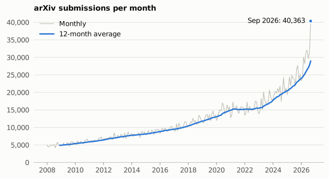
Through the 2010s arXiv grew by 5 to 14 percent a year, and it nearly stalled in 2021 and 2022. The first eight months of `{python} Y1` grew `{python} K['yoy']`, after `{python} K['yoy_prev']` the year before. `{python} K['sep_month']`, the latest complete month in arXiv's own statistics, brought `{python} K['sep']` submissions, `{python} K['sep_x']` times the figure of two years earlier. The "lift-off" in the LinkedIn post is not a plotting artefact.
::: {.thorough}
Year-over-year growth for the same January to `{python} LAST.strftime('%B')` window, from the per-paper table:
```{python}
#| label: yoy-table
pd.DataFrame({"papers": n, "growth": yoy}).loc[2016:].style.format({"papers": "{:,}", "growth": "{:+.1%}"})
```
:::
## Where the growth comes from
```{python}
#| label: fig-fields
#| fig-cap: "Papers added between the two January to August windows, by subject group and by primary category."
fig, axes = plt.subplots(1, 2, figsize=(9.2, 4.2), gridspec_kw={"wspace": 0.55})
names = {"cs": "Computer science", "physics": "Physics", "math": "Mathematics", "stat": "Statistics",
         "econ": "Economics", "eess": "Electrical eng.", "q-fin": "Quant. finance", "q-bio": "Quant. biology"}
for ax, t, title, lab in [(axes[0], g_group, "By subject group", lambda i: names[i]),
                          (axes[1], g_cat.head(10), "Top 10 categories", str)]:
    t = t.iloc[::-1]
    ax.barh([lab(i) for i in t.index], t["added"], color=BLUE, height=0.62)
    for y, (a, g) in enumerate(zip(t["added"], t["growth"])):
        ax.text(max(a, 0), y, f"  {a:+,} ({g:+.0%})", va="center", ha="left", color=INK2, fontsize=9)
    ax.set_title(title); ax.grid(False); ax.set_xticks([]); ax.spines["bottom"].set_visible(False)
    ax.set_xlim(min(0, t["added"].min()), t["added"].max() * 1.75); ax.tick_params(length=0)
fig.suptitle(f"Papers added, Jan to {LAST.strftime('%b')} {Y0} vs {Y1} (growth in brackets)", x=0.02, ha="left", fontsize=10, color=INK2)
plt.show()
```
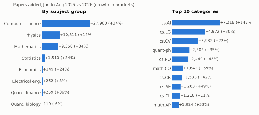
Computer science accounts for `{python} K['cs_share']` of the added papers, and one category stands out: cs.AI grew `{python} K['ai_x']`x in a single year. arXiv singled out the same category when it [introduced submission rate limits on 1 October 2026](https://blog.arxiv.org/2026/10/01/updated-rate-limit-policy/).
The more surprising result is outside CS. Mathematics grew `{python} K['math_g']` and physics `{python} K['phys_g']`, in fields that had been growing by a few percent a year. Combinatorics (math.CO) grew faster than computer vision. A surge that reaches pure mathematics is not explained by "more people are working on AI". Something changed in how quickly papers get written across fields.
::: {.thorough}
The full group table is in Step 6. The twenty categories that added the most papers:
```{python}
#| label: categories-table
g_cat.head(20).style.format({"growth": "{:+.1%}", "share of growth": "{:.1%}", Y0: "{:,}", Y1: "{:,}", "added": "{:+,}"})
```
:::
## Which countries and institutions
```{python}
#| label: fig-geo
#| fig-cap: "Implied growth in papers from January to August 2024 to the same months of 2026, from weighted samples of about 9,000 affiliated papers per year. Bars are 95% bootstrap intervals; the dashed line is arXiv's total growth. Tiers use each paper's best-ranked university in the Leiden Ranking Open Edition 2025."
CNAMES = {"US": "United States", "CN": "China", "DE": "Germany", "GB": "United Kingdom", "JP": "Japan", "FR": "France",
          "IN": "India", "CA": "Canada", "IT": "Italy", "KR": "South Korea", "ES": "Spain", "AU": "Australia",
          "HK": "Hong Kong", "CH": "Switzerland", "NL": "Netherlands"}
fig, axes = plt.subplots(1, 2, figsize=(9.2, 4.4), gridspec_kw={"wspace": 0.7, "width_ratios": [1, 1.1]})
for ax, t, title, lab in [(axes[0], g_tier, "By institution tier", str),
                          (axes[1], g_country.sort_values("growth"), "By country (fractional)", lambda c: CNAMES.get(c, c))]:
    t = t.iloc[::-1] if t is g_tier else t
    y = np.arange(len(t))
    ax.hlines(y, t["low"], t["high"], color="#c3c2b7", lw=2.5)
    ax.scatter(t["growth"], y, color=BLUE, s=28, zorder=3, edgecolor="#fcfcfb", linewidth=1.2)
    ax.axvline(growth_all - 1, color=MUTED, lw=1, ls=(0, (3, 3)))
    ax.set_yticks(y, [f"{lab(i)}  {s:.0%}" for i, s in zip(t.index, t[f"share {Y1}"])])
    ax.xaxis.set_major_formatter(pct0); ax.set_xlim(0, 1.3); ax.grid(axis="x"); ax.grid(axis="y", visible=False)
    ax.set_title(title); ax.tick_params(length=0)
fig.suptitle(f"Growth {Ya} to {Y1}, with each group's {Y1} share of papers", x=0.02, ha="left", fontsize=10, color=INK2)
plt.show()
```
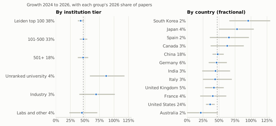
One commenter asked whether growth was uniform across university rankings. It was, to a degree that is easy to miss on the chart. Over the two years from `{python} Ya` to `{python} Y1` arXiv grew `{python} K['geo_all']`. Papers with an author at one of the Leiden top 100 grew `{python} K['t100']` (95 percent interval `{python} K['t100_lo']` to `{python} K['t100_hi']`). The 101 to 500 tier grew `{python} K['t500']`, and everything ranked below 500 grew `{python} K['t501']`. Ranked universities supply `{python} K['ranked_share']` of affiliated papers, and they supplied `{python} K['ranked_growth_share']` of the growth. The top 100's share slipped from `{python} K['t100_s0']` to `{python} K['t100_s1']`, which is about as small a change as this sample can detect.
The fastest growth sits at the margins. Papers whose best affiliation is a university outside the ranking grew `{python} K['t_unr']` (interval from `{python} K['t_unr_lo']`, clearly above arXiv's overall rate), and papers with company authors but no ranked university grew `{python} K['t_ind']` (from `{python} K['t_ind_lo']`, so not clearly faster). Both are small groups: unranked universities went from `{python} K['t_unr_share0']` to `{python} K['t_unr_share1']` of papers. Industry as a whole did not gain ground: the share of papers with at least one company author went from `{python} K['ind0']` to `{python} K['ind1']`.
Geographically, the surge is not one country's story either. The United States grew `{python} K['us_g']`, a little slower than arXiv, and China `{python} K['cn_g']`; between them they supplied `{python} K['us_gs']` and `{python} K['cn_gs']` of the added papers. South Korea (`{python} K['kr_g']`) and Japan (`{python} K['jp_g']`) grew fastest among the large contributors.
Where the tiers *do* differ is in how they write. Solo papers are rare at top universities and common outside them, and the solo share rose everywhere. In the top 100 it went from `{python} K['solo_t100_0']` to `{python} K['solo_t100_1']`. Among unranked universities it went from `{python} K['solo_unr_0']` to `{python} K['solo_unr_1']`.
::: {.thorough}
Growth by tier under both rankings, and the weighted solo-author share by tier. The two rankings disagree about which universities are "top 100" (the share ranking has fewer large Chinese universities and more British and Dutch ones), but they agree that the tiers grew at about the same rate.
```{python}
#| label: geo-tables
fmt = {f"share {Ya}": "{:.1%}", f"share {Y1}": "{:.1%}", "growth": "{:+.0%}", "low": "{:+.0%}", "high": "{:+.0%}", "share of growth": "{:.1%}"}
display(pd.concat({"Ranked by number of top-10% papers": g_tier,
                   "Ranked by share of top-10% papers (3,000+ papers)": g_tier_share}).style.format(fmt))
display(solo_by_tier.style.format("{:.1%}"))
g_country.rename(index=CNAMES).style.format(fmt)
```
Coverage is the main caution. Only papers OpenAlex can attach affiliations to are in the sample, about half of 2024's papers and two thirds of 2026's. Reweighting fixes the subject and team-size mix but not anything else that decides whether OpenAlex finds an affiliation. 2025 is left out because OpenAlex's coverage of it is too patchy to use.
:::
## Who is submitting more
```{python}
#| label: fig-who
#| fig-cap: "Left: papers per submitting account within each January to August window. Right: which accounts supplied the growth."
fig, axes = plt.subplots(1, 2, figsize=(9.2, 3.8), gridspec_kw={"wspace": 0.3})
ax = axes[0]
pps = per_year["papers per submitter"]
ax.plot(pps.index, pps.values, color=BLUE, marker="o", ms=5, markeredgecolor="#fcfcfb")
ax.annotate(f"{pps.iloc[-1]:.2f}", (pps.index[-1], pps.iloc[-1]), xytext=(-6, 4), textcoords="offset points", ha="right")
ax.set_ylim(1.3, 1.65); ax.set_title("Papers per account"); ax.set_xticks(range(2015, Y1 + 1, 2))
ax = axes[1]
ax.bar(g_tenure.index.astype(str), g_tenure["share of growth"], color=BLUE, width=0.55)
for i, v in enumerate(g_tenure["share of growth"]):
    ax.text(i, v + 0.01, f"{v:.0%}", ha="center", color=INK)
ax.yaxis.set_major_formatter(pct0); ax.set_ylim(0, 0.6); ax.set_title(f"Share of {Y0} to {Y1} growth, by account age")
plt.show()
```
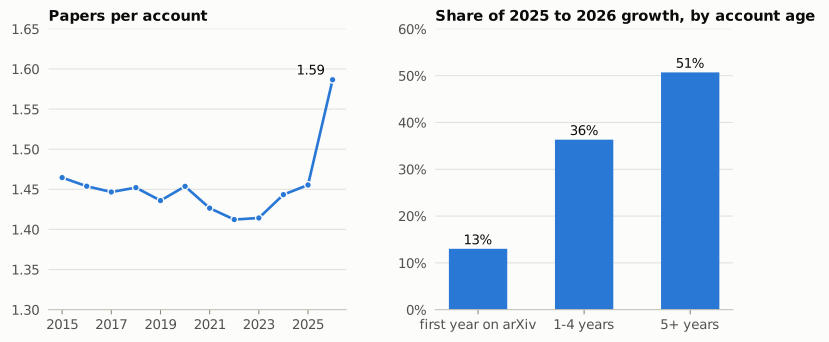
If paper mills or first-time hobbyists were driving the surge, new accounts would dominate the growth. They do not. Accounts in their first year supplied `{python} K['debut_share']` of the added papers, and their output grew more slowly than anyone else's, which fits arXiv's [tightened endorsement rules for new submitters](https://blog.arxiv.org/2026/01/21/attention-authors-updated-endorsement-policy/) in January 2026. Half of the growth (`{python} K['vet_share']`) came from accounts that have been on arXiv for five years or more.
What changed is the pace. For ten years the average account submitted about 1.45 papers in an eight-month window, almost without variation. In `{python} Y1` that rose to `{python} K['pps1']`. The people who were already writing papers are writing more of them.
::: {.thorough}
The three splits behind this section. Accounts that submitted five or more papers in the window are where output grew fastest:
```{python}
#| label: who-table
fmt = {"growth": "{:+.1%}", "share of growth": "{:.1%}", Y0: "{:,}", Y1: "{:,}", "added": "{:+,}"}
pd.concat({"Account age": g_tenure, "Authors on the paper": g_team, "Papers by the account in the window": g_volume}).style.format(fmt)
```
:::
## The solo-author break
```{python}
#| label: fig-solo
#| fig-cap: "Left: share of new papers with a single author, by month. Right: accounts that submitted five or more single-author papers in a January to August window."
fig, axes = plt.subplots(1, 2, figsize=(9.2, 3.8), gridspec_kw={"wspace": 0.3})
ax = axes[0]
sm = monthly["solo"].rolling(3).mean()
ax.plot(sm.index.to_timestamp(), sm.values, color=BLUE)
ax.yaxis.set_major_formatter(pct0); ax.set_ylim(0, 0.25); ax.set_title("Single-author share (3-month average)")
ax = axes[1]
sp = solo_prolific["accounts with 5+ solo papers"]
ax.bar(sp.index, sp.values, color=BLUE, width=0.62)
ax.text(sp.index[-1], sp.iloc[-1] + 8, f"{sp.iloc[-1]:,}", ha="center"); ax.text(sp.index[-2], sp.iloc[-2] + 8, f"{sp.iloc[-2]:,}", ha="center")
ax.set_title("Accounts with 5+ solo papers"); ax.set_xticks(range(2015, Y1 + 1, 2))
plt.show()
```
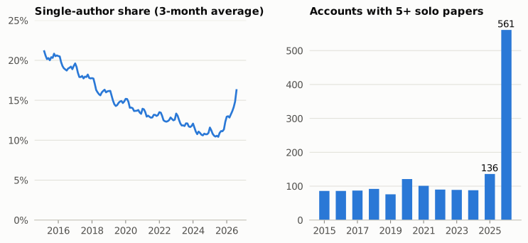
This is the clearest structural break in the data. Research had been getting steadily more collaborative: the single-author share of new papers fell from about 20 percent in 2015 to under 11 percent in 2025. In `{python} Y1` it turned around. Single-author papers grew `{python} K['solo_g']` while multi-author papers grew `{python} K['multi_g']`, and solo papers alone account for `{python} K['solo_share']` of all the growth.
At the extreme end is the pattern Srijit described. The number of accounts posting five or more single-author papers in eight months sat around 100 for a decade, reached `{python} K['sp0']` in `{python} Y0`, and then `{python} K['sp1']` in `{python} Y1`. One person producing a paper every few weeks, alone, was rare enough to be a curiosity. It no longer is.
It is also a small part of the whole. Their solo papers number `{python} K['sp_papers']`, or `{python} K['sp_pct']` of the window. arXiv's new cap of two submissions per account per month would have held back `{python} K['cap1']` of `{python} Y1`'s papers (it was `{python} K['cap0']` the year before). The high-frequency tail is real and growing fast, but removing it entirely would leave nearly all of the surge in place.
::: {.thorough}
```{python}
#| label: solo-table
per_year.join(solo_prolific).join(over_cap.rename("share above 2/month")).style.format({
    "papers": "{:,}", "submitters": "{:,}", "papers per submitter": "{:.3f}", "share from 5+ accounts": "{:.1%}",
    "solo share": "{:.1%}", "papers from 5+ solo accounts": "{:,}", "share above 2/month": "{:.1%}"})
```
No accounts are named here on purpose. A submitter name is not proof of anything: prolific legitimate accounts exist (proceedings series, large collaborations), and common names merge several people.
:::
## Do solo authors cite themselves?
```{python}
#| label: fig-selfcite
#| fig-cap: "Left: share of references in each paper's bibliography that include one of its own authors (January to August 2026 papers). Right: for papers first posted January to August 2025 and cited at least once in their first year, the average share of those citations from the paper's own authors. Bars run from matching on Semantic Scholar author ids (lower end) to ids or surname plus initial (upper end)."
LAB = {"solo": "Single-author", "prolific solo": "Prolific solo accounts\n(5+ solo papers)", "multi": "Multi-author"}
fig, axes = plt.subplots(1, 2, figsize=(9.2, 3.6), gridspec_kw={"wspace": 0.15})
ax = axes[0]
t = selfref.xs(Y1, level="year").iloc[::-1]
y = np.arange(len(t))
ax.hlines(y, t["self-citation share (id)"], t["self-citation share (id or name)"], color=BLUE, lw=7, alpha=0.85)
for i, (lo, hi) in enumerate(zip(t["self-citation share (id)"], t["self-citation share (id or name)"])):
    ax.text(hi + 0.006, i, f"{lo:.0%} to {hi:.0%}", va="center", color=INK2, fontsize=9)
ax.set_yticks(y, [LAB[s] for s in t.index]); ax.set_xlim(0, 0.2); ax.xaxis.set_major_formatter(pct0)
ax.set_title("Self-citations among references"); ax.grid(axis="x"); ax.grid(axis="y", visible=False); ax.tick_params(length=0)
ax = axes[1]
t = impact_12m.xs(Y0, level="year").reindex(selfref.xs(Y1, level="year").index).iloc[::-1]
ax.barh(y, t["self_citation_fraction"], color=ORANGE, height=0.5)
for i, (v, o) in enumerate(zip(t["self_citation_fraction"], t["cited_only_by_own_authors"])):
    ax.text(v + 0.01, i, f"{v:.0%}  ({o:.0%} cited only by themselves)", va="center", color=INK2, fontsize=9)
ax.set_yticks(y, []); ax.set_xlim(0, 1); ax.xaxis.set_major_formatter(pct0)
ax.set_title("Self-citations among first-year citations"); ax.grid(axis="x"); ax.grid(axis="y", visible=False); ax.tick_params(length=0)
plt.show()
```
Another reader asked whether most single-author papers are self-citations, which can mean two things. Do solo papers mostly cite the author's own earlier work? And are the citations they receive mostly from the author?
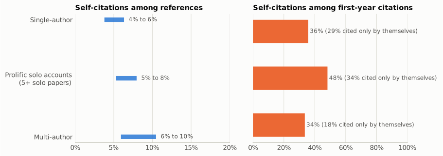
On the first, the answer is a clear no. In the `{python} Y1` sample a single-author paper has a median of `{python} K['sr_refs']` references, and `{python} K['sr_solo']` to `{python} K['sr_solo_hi']` of them include the author, depending on how strictly names are matched. That is *lower* than for multi-author papers (`{python} K['sr_multi']` to `{python} K['sr_multi_hi']`), which have more authors whose past work can be cited. Only `{python} K['sr_major']` of solo papers have a bibliography that is mostly self-citation, and the share that cite no earlier work of the author's at all rose from `{python} K['sr_none0']` in `{python} Y1 - 2` to `{python} K['sr_none1']`. That fits a wave of solo papers by people writing outside their own track record. It does not fit people padding their citation counts. Even the prolific solo accounts sit at `{python} K['sr_pro']` to `{python} K['sr_pro_hi']`.
The second reading is where self-citation shows up. Of single-author papers posted in `{python} Y0`, those cited at all in their first year got on average `{python} K['sf_solo']` of those citations from their own author, and `{python} K['os_solo']` were cited by nobody else. Multi-author papers are similar on the first measure (`{python} K['sf_multi']`) but less often cited only by themselves (`{python} K['os_multi']`). The prolific solo accounts stand out: `{python} K['sf_pro']` of their early citations are their own, and `{python} K['os_pro']` of their cited papers are cited by no one else. A person posting a paper every few weeks naturally builds on the last one, so this is not misconduct in itself. It does mean that raw citation counts flatter this group more than any other.
::: {.thorough}
References. `self-citation share` pools all references in the stratum; `median_self_share` is the per-paper median; `majority_self` is the share of papers whose references are more than half self-citations; `no_self` is the share with none. Author ids and names are matched as described in Step 8.
```{python}
#| label: selfcite-table
selfref.style.format({"median_refs": "{:.0f}", "median_self_share": "{:.1%}", "majority_self": "{:.1%}", "no_self": "{:.1%}",
                      "self-citation share (id)": "{:.1%}", "self-citation share (id or name)": "{:.1%}"})
```
:::
## Are credible venues growing the same way?
```{python}
#| label: fig-venues
#| fig-cap: "Output over February to August of each year, indexed to 2023. Crossref counts are journal articles by publication date."
base = Y1 - 3
idx = venues.loc[base:] / venues.loc[base] * 100
fig, ax = plt.subplots(figsize=(7.6, 4.0))
for col, c in zip(idx.columns, [BLUE, ORANGE, AQUA, YELLOW]):
    ax.plot(idx.index, idx[col], color=c, marker="o", ms=5, markeredgecolor="#fcfcfb", label=col)
    ax.annotate(f"{col}  {idx[col].iloc[-1]:.0f}", (Y1, idx[col].iloc[-1]), xytext=(8, 0), textcoords="offset points", va="center", color=INK)
ax.set_xticks(idx.index); ax.set_xlim(base - 0.15, Y1 + 1.6); ax.set_ylim(95, None)
ax.legend(loc="upper left"); ax.set_title(f"Growth since {base} ({base} = 100)")
plt.show()
```
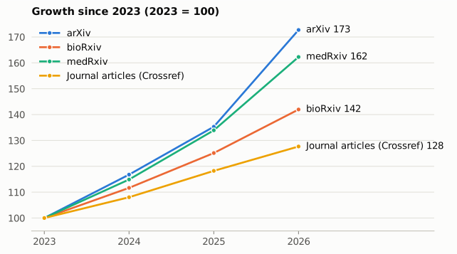
This was the test proposed in the comments, and the answer is no. Over three years arXiv grew about `{python} f"{venue_growth.iloc[0, 1]:.0%}"`, while journal articles registered with Crossref grew `{python} f"{venue_growth.iloc[3, 1]:.0%}"`. In the latest year arXiv grew `{python} K['arx']` against `{python} K['jrn']` for journals. The life-science preprint servers sit in between. medRxiv comes closest, at `{python} K['med']` in the latest year, but it is a twentieth of arXiv's size and was already growing almost that fast; neither server shows a jump in `{python} Y1` like arXiv's.
Two cautions. Crossref counts every journal with a DOI, so "credible, defined broadly" is doing a lot of work, and journal growth includes paper-mill output of its own. And journals lag preprints: a paper posted in 2026 may be published in 2027. A gap this wide still means that preprints are being produced far faster than the peer-review system is currently absorbing them. Either a wave of publications is on its way, or a growing share of arXiv will never be reviewed by anyone.
::: {.thorough}
```{python}
#| label: venues-table
venues.style.format("{:,}")
```
:::
## Is the new work being used?
```{python}
#| label: fig-impact
#| fig-cap: "Share of papers cited at least once, counting only citing papers dated within 6 or 12 months of the paper's first version. The 12-month comparison covers January to August cohorts; the 6-month view of 2026 covers only papers posted by early March, the youngest old enough to measure."
fig, axes = plt.subplots(1, 2, figsize=(9.2, 3.6), gridspec_kw={"wspace": 0.25})
for ax, t, title, years in [(axes[0], impact_12m, "Cited within 12 months", [Y1 - 2, Y0]),
                            (axes[1], impact_6m, "Cited within 6 months", [Y1 - 2, Y0, Y1])]:
    u = t["cited"].unstack("year").reindex(ORDER)
    width = 0.8 / len(years)
    for k, (yr, c) in enumerate(zip(years, [MUTED, BLUE, ORANGE])):
        xs = np.arange(len(u)) + (k - (len(years) - 1) / 2) * width
        ax.bar(xs, u[yr], width=width * 0.92, color=c, label=str(yr))
        for x_, v in zip(xs, u[yr]):
            if v == v:
                ax.text(x_, v + 0.01, f"{v:.0%}", ha="center", fontsize=8, color=INK2)
    ax.set_xticks(np.arange(len(u)), [{"solo": "Single-author", "prolific solo": "Prolific solo\naccounts", "multi": "Multi-author"}[s]
                                      for s in u.index], fontsize=9)
    ax.yaxis.set_major_formatter(pct0); ax.set_ylim(0, 0.85); ax.set_title(title); ax.legend(loc="upper left", ncol=3)
plt.show()
```
The most useful long-run suggestion from the comments was to track which preprints become journal papers, then compare citations from inside and outside the paper's field, since work that travels across fields tends to matter more. As the commenter said, that needs a couple of years. What can be done now is a fair early comparison: count each cohort's citations at the same age, so that older papers are not flattered simply for having had longer to collect them.
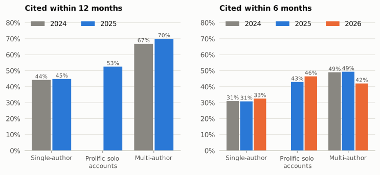
On that basis, the first surge cohort looks like the one before it. `{python} Y0`'s growth (`{python} K['yoy_prev']`) was smaller than `{python} Y1`'s, but already at the top of the 2010s range. Within 12 months, `{python} K['ci_solo1']` of its single-author papers had been cited at least once, against `{python} K['ci_solo0']` for `{python} Y1 - 2`. For multi-author papers the figures are `{python} K['ci_multi1']` and `{python} K['ci_multi0']`. Prolific solo accounts are cited *more* often than other solo authors (`{python} K['ci_pro']`), but as the previous section showed, much of that is self-citation. Citations that cross fields are rare for everyone in the first year: `{python} K['out_solo']` of cited solo papers and `{python} K['out_multi']` of cited multi-author papers drew at least one citation from outside their broad discipline.
The `{python} Y1` cohort can only be seen at six months, and only for papers posted between January and early March (`{python} K['c6_n']` papers in the sample). `{python} K['c6_solo']` of its solo papers had been cited by then (`{python} Y0`: `{python} K['c6_solo0']`), and `{python} K['c6_multi']` of multi-author papers (`{python} Y0`: `{python} K['c6_multi0']`). The multi-author dip may be indexing lag rather than lower use, since these are the citations Semantic Scholar has had the least time to find. Either way, neither a collapse nor a boom in early uptake is visible yet.
This is the measurement to repeat. In a year the full `{python} Y1` cohort will have 12-month citations, and by 2028 two-year windows plus journal publication will be observable. Those windows are long enough to look properly at citations from outside the field.
::: {.thorough}
Per-paper measures, every paper weighted equally. `mean_citations_capped_20` caps each paper at 20 so that one runaway paper cannot move the average (one 2024 solo paper in the sample collected 2,365 citations in a year). The self-citation and outside-field columns are among papers cited at least once.
```{python}
#| label: impact-tables
fmt = {"papers": "{:,}", "cited": "{:.1%}", "mean_citations_capped_20": "{:.2f}", "self_citation_fraction": "{:.1%}",
       "cited_only_by_own_authors": "{:.1%}", "any_outside_field_citation": "{:.1%}"}
display(impact_12m.style.format(fmt).set_caption("Within 12 months"))
impact_6m.style.format(fmt).set_caption("Within 6 months")
```
:::
## What the abstracts can and cannot tell us
```{python}
#| label: fig-marker
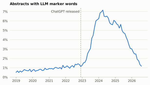
#| fig-cap: "Share of new abstracts using at least one of: delve, underscore, showcase, pivotal, intricate, meticulous (any inflection)."
mk = monthly["marker"].loc["2019-01":]
fig, ax = plt.subplots()
ax.plot(mk.index.to_timestamp(), mk.values, color=BLUE)
ax.axvline(pd.Timestamp("2022-11-30"), color=MUTED, lw=1, ls=(0, (3, 3)))
ax.text(pd.Timestamp("2022-11-01"), mk.max(), "ChatGPT released ", ha="right", va="top", color=INK2)
ax.yaxis.set_major_formatter(pct0); ax.set_ylim(0); ax.set_title("Abstracts with LLM marker words")
plt.show()
```
An obvious idea is to detect AI-written text directly. Researchers have done this through "excess vocabulary": words such as *delve* that became abruptly more common after ChatGPT appeared ([Kobak et al.](https://arxiv.org/abs/2406.07016)). The same handful of words in arXiv abstracts shows the rise clearly, peaking at `{python} K['marker_peak']` of abstracts in `{python} K['marker_peak_m']`.
Then it falls away, back to `{python} K['marker_now']` by `{python} LAST.strftime('%B %Y')`, during the exact period when submissions took off. Nobody believes LLM use declined in 2026. Models changed their habits and authors learned to edit out the tells. A fixed word list is a detector for one generation of models, and it says nothing about quality in any case: a careful paper polished by an LLM and a fabricated one both trip it.
Abstracts did get longer, though: the median went from `{python} f"{monthly.abs_words.loc[f'{Y0}-01':f'{Y0}-08'].median():.0f}"` words in early `{python} Y0` to `{python} f"{monthly.abs_words.iloc[-3:].median():.0f}"` by mid `{python} Y1`, after creeping up by a word or two a year.
::: {.thorough}
### Why publication status cannot settle it yet
The natural quality measure is whether a preprint ends up published. The snapshot has three signals: a journal reference, a DOI, and comments mentioning acceptance. All three are added *after* the fact, so recent cohorts always look worse than old ones regardless of quality:
```{python}
#| label: censoring-table
c = W.groupby("year").agg(journal_ref=("has_jref", "mean"), doi=("has_doi", "mean"), accepted_in_comments=("accepted", "mean"))
c.loc[2018:].style.format("{:.1%}")
```
The decline starts years before the surge and steepens toward the present, which is what right-censoring looks like. Comparing cohorts fairly needs each one measured at the same age, which means keeping successive snapshots. That is the follow-up worth doing: re-run this notebook in a year and compare the `{python} Y1` cohort's publication rate at twelve months with the `{python} Y0` cohort's today.
:::
## So: acceleration or slop?
The data rule out the simple version of each story.
It is not a flood of outsiders and mills. The growth comes mainly from people with a track record on arXiv, across computer science, mathematics and physics at once, at top universities about as much as anywhere else, and the accounts that behave like mills are a few percent of the total at most.
It is also not business as usual at higher speed. Papers per account jumped after a decade of stability, solo work reversed a long decline, and peer-reviewed output did not move with it. The same researchers are producing papers faster than before, increasingly alone, and faster than journals and conferences are certifying them.
Whether that is acceleration of *research* or only of *papers* is not something titles, author lists and abstracts can decide. arXiv's moderators, who read the submissions, describe a rise in ["thin papers of narrow scope"](https://blog.arxiv.org/2026/10/01/updated-rate-limit-policy/) and work split into smaller pieces, and have responded with endorsement rules and rate limits. The measurements that would settle it are outcomes: what share of the `{python} Y1` cohort is published a year on, how it is cited and by whom, inside and outside its field, and how often it is withdrawn. The first look shows no drop: the `{python} Y0` cohort was taken up as quickly as the one before it. The full `{python} Y1` cohort can be measured properly from 2027.
## Limitations {.thorough}
- **Submitter names are not identities.** The snapshot has display names, not account IDs. Common names merge several people and inflate "papers per account"; a person who changes their display name is split. This affects every year, but collisions grow with volume, so the level of the prolific-account counts is less reliable than their direction. The solo-author share does not depend on names at all.
- **Account age is measured from the first paper under that name** in the snapshot, with the same caveat.
- **The comparison window is January to `{python} LAST.strftime('%B')`.** `{python} K['sep_month']` appears only in the official monthly count; the per-paper snapshot was taken before that month ended.
- **Crossref dates are publication dates as deposited by publishers.** Year-only dates land on 1 January (excluded here), and recent months can still gain records as publishers deposit late, which would slightly understate journal growth.
- **Primary category only.** Cross-listed papers are counted once, under their first category.
- **No full text and no moderation data.** Rejected submissions never appear in the snapshot, so this is the growth that survived arXiv's moderation.
- **Affiliations are a reweighted sample, two years apart.** OpenAlex attaches affiliations to roughly half to two thirds of arXiv papers, and its 2025 coverage is too patchy to use, so the geography section compares `{python} Y1 - 2` with `{python} Y1` rather than the latest year. Reweighting corrects the subject and team-size mix but not any other reason a paper's affiliations go missing.
- **Leiden ranks are not QS ranks.** The tiers use an open, citation-based ranking. QS also weighs reputation surveys, staff ratios and internationalisation. Both rankings favour large research universities. Treat "top 100" here as "most highly cited output", not as an equivalent of QS.
- **Self-citation depends on author matching.** Semantic Scholar's author ids miss self-citations when one person is split across profiles. Matching on surname and first initial catches those but over-counts common names. The truth lies between the two columns.
- **Citations are from Semantic Scholar's index**, which covers arXiv and most journals but not books or most patents, and adds recent citing papers with a lag of a few weeks.
## Reproducing this {.thorough}
```bash
conda env create -f environment.yml && conda activate arxiv-analysis
quarto render arxiv-liftoff.qmd
```
The first render downloads about 1.8 GB and takes several minutes to parse; later renders reuse `data/` and finish in seconds. Delete `data/raw/` to refresh every source.